Introduction
Diabetic Retinopathy(DR) damages the blood vessels within the retinal tissue, resulting in fluid leakage and distorted vision. DR progresses in four stages. We aim to build a deep-learning-based method for stage detection of diabetic retinopathy on a single picture of the human fundus. Additionally, we will compare the different supervised ML methods with deep learning-based CNN approach. We will be using datasets provided by APTOS and Kaggle for this project.[2]
Literature Review
The growing popularity of deep learning-based approaches in diabetic retinopathy diagnosis has led to various methods employing Convolutional Neural Networks (CNNs). Pratt et al. (2016)[3] developed a CNN-based network with data augmentation and achieved a sensitivity of 95% and an accuracy of 75% on 5,000 validation images. Other researchers, such as Sarki et al.[4], tried to train ResNet50, Xception Nets, DenseNets and VGG with ImageNet and achieved an accuracy of 81.3%.
Other researchers, such as Carson Lam and Lindsey (2018)[5] and Yung-Hui Li and Chung (2019)[6], have also explored CNNs for this purpose. Asiri et al. (2018)[7] reviewed multiple methods and datasets, highlighting their advantages and disadvantages and pointing out challenges and future research directions. Diabetic retinopathy is a serious diabetic complication affecting the blood vessels in the eyes of patients. Over time, high blood sugar levels damage these vessels, leading to vision impairment and even blindness. Regular eye exams are crucial in preventing and treating this sight-threatening condition. In our attempt to improve diagnostic rates for DR, we propose creating supervised models to train
Additionally, transfer learning with CNN architectures has been investigated. Hagos et al. (2019)[8]trained InceptionNet V3 with pretraining on the ImageNet dataset, achieving an accuracy of 90.9% in 5-class classification. Sarki et al. (2019)[4] trained ResNet50, Xception Nets, DenseNets, and VGG with ImageNet pretraining, achieving the highest accuracy of 81.3%. Both research teams utilized datasets provided by APTOS and Kaggle for their studies.
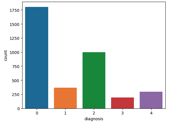
Description of Dataset
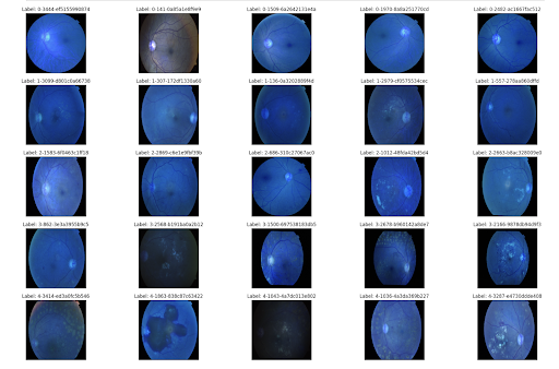
In this project, we are using a kaggle dataset. The data was collected from multiple clinics using a variety of cameras over an extended period of time, which will introduce further variation. Each image is an image of an eyeball of potential patients of diabetic retinoscopy. The classes in which the images are divided based on the severity of the condition are: 0: No DR 1: Mild 2: Moderate 3: Severe 4: Proliferate DR We have a total of 3662 images in our dataset. For each image we have an id_code and a diagnosis value which is equivalent to the classes described above. The distribution of the data is as follows:
Link of Dataset
The Dataset Link is : https://www.kaggle.com/competitions/aptos2019-blindness-detection/data
Problem Definition and Motivation
Diabetic Retinopathy is one of the leading causes of blindness and eye disease in the working age population of the developed world. This project is an attempt towards developing a machine learning project for detection using supervised and unsupervised techniques to detect this disease in early phase. For the project, use of these methods on retinal fundus images is done to classify a given set of images into stages of DR. DR is a condition that may occur in diabetic people causing increasing damage to the retina of affected eye. Research shows that it contributes 4.8% of total cases of blindness.[1]

Image source: https://www.dreamstime.com/stock-images-diabetic-retinopathy-image20016314
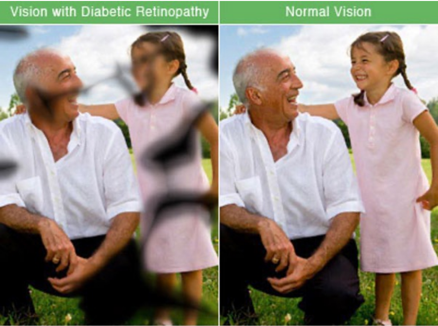 Image source: https://www.daily-mail.co.zm/diabetic-retinopathy-one-leading-blindness-causes/
Methods:
Data Pre-processing
Our classification depends heavily on how clearly we can see the spots inside the eyeball and thus color contrast plays a huge role in it. To check whether we have any dark images in our dataset we use 2 techniques:
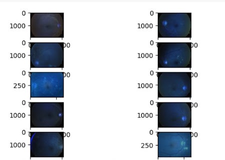
- Standard Deviation of the pixels : For each image, we calculate the standard deviation of the pixel values to get a measure of the contrast. To test this technique we manually take a few images which would have been categorized as bad data points and equal number of good data points and calculate the standard deviation for each of them. Through trial and error, it was concluded that images with a standard deviation below 16 should be discarded. In our dataset of ~3650 images, 100 images were categorized to be discarded.A few images that had low standard deviation:
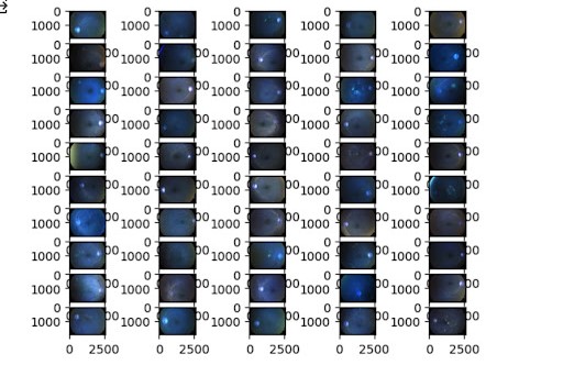
- KMeans : We also decided to use KMeans to potentially cluster darker images together which would then be discarded. By running the algorithm for K = 7, we did get a cluster with relatively darker images but a few of the images within the cluster were still acceptable. Additionally the size of the cluster was >100 and discarding images at this scale was not feasible. A section of the described cluster:
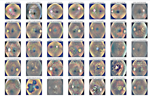
Instead of discarding the dark images, we wanted to improve the color contrast to not lose on data. To do this and add uniformity to the dataset we followed the following steps:
- Crop out the dark parts from the image: We check the pixel values in a given image and if it is below a certain threshold (on the grayscale) then we mark that pixel as invalid. If most of the image is dark we return the original image otherwise return the valid pixel images in the form of a cropped image.
- Resize the image: After cropping out, the images are resized to a predefined size (such as 256x256)
- Increase contrast in the image: A weighted sum of the original image and a Gaussian-blurred version is taken to enhance the light portions and decrease the intensity of the darker regions.
After following the above steps we see a clear difference in the images and can observe the eyeballs more clearly.
To verify the results, we again check the standard deviation of the pixels and run KMeans. With standard deviation we only get 9 images below the set threshold of 16 and with KMeans we get a small cluster of ~10 images that are still dark. We discarded these.
Principal Component Analysis (PCA)
Our preprocessed dataset consists of images of size (256, 256, 3), where 3 refers to the 3 channels (Red, Green, Blue). So, for each channel we can consider there to be 65536 features, which is a lot for simpler models to handle.
We use PCA, a popular technique to reduce dimensions (features) in larger datasets. PCA attempts to reduce features by retaining as much information as possible. It selects features that account for the maximum possible variance in the data set.
We have tried three ways of using dimensionality reduction with PCA:
- We convert the dataset to grayscale and flatten it to get a (3662, 65536) input array. We then run PCA to get features that retain 95 and 99% of the variance, which we used to train our logistic regression model.
As we came up with better preprocessing steps we discarded results from this approach. - Since the PCA function in scikit-learn works with only 2D input arrays, and recognising the importance of keeping the colour information, we chose to run PCA on each colour channel separately and then merge it.
We observe that to retain 95% of the variance, each channel needs a different number of features: Red: 873; Green: 1379; Blue: 1551; so we decided to retain the maximum among the three.
Training with this dataset, we realise that the number of features is very high when compared to the size of our input. This method was overfitting our dataset, so we decided to discard this approach. - Finally, we use PCA on the preprocessed dataset after converting it to grayscale. To retain 95% of the variance in this scenario, we need 1092 features.
Models Implemented
Logistic Regression (Supervised)
We perform logistic regression on the output of PCA (performed on the grayscale images) that retains 95% of the variance. This was chosen over the data retaining 99% variance to reduce the chances of overfitting due to the larger number of features present when compared to the number of datapoints. The input data had 3662 samples and 1092 features. The data is standardized (by subtracting the mean and dividing by the standard deviation for each feature of the input data) before being split into training and test data sets. We use a 80-20 rain to test ratio. Logistic regression is then performed using a one-vs-rest strategy (default threshold of 0.5 is retained).
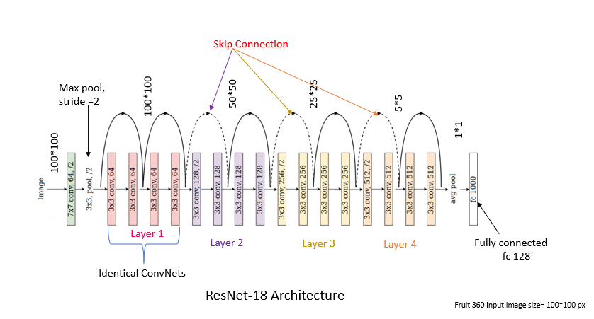
CNN - Resnet18 (Supervised)
We use a popular CNN architecture - Resnet18 (18 layers deep), designed for image classification, and train it on the original cleaned dataset (before PCA). The Resnet architecture introduces skip connections that directly connect earlier layers to later layers. This mitigates the vanishing gradient problem. We used the Resnet18 architecture without the pre-loaded weights (from training on the ImageNet dataset) and trained it using our dataset (80-10-10 train to validation to test split).
CNN - VGGNet16 (Supervised)
Another popular CNN architecture - VGGNet16 (16 layers deep) is tested. This time, the model was loaded with the pretrained weights from the ImageNet dataset (which consists of more than a million images), which can classify images into 1000 object categories. The top layer was removed and replaced with 3 fully connected layers, with the last layer having 5 outputs to match the number of classes. The training was then performed for 20 epochs, using our cleaned dataset (80-10-10 train to validation to test split).
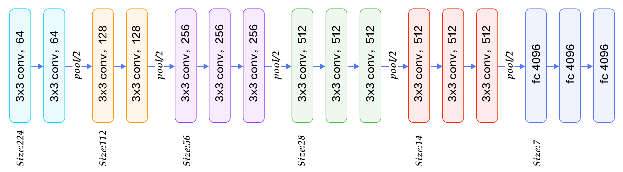
Image source: https://raw.githubusercontent.com/blurred-machine/Data-Science/master/Deep%20Learning%20SOTA/img/network.png
CNN - Inception-v3 (Supervised)
Inception refers to a series of convolutional neural network (CNN) architectures developed by Google for image recognition tasks. The name “Inception” comes from the concept of having “inception modules” within the architecture, which are modules that capture information at multiple scales. The fundamental idea of an Inception module is to use multiple filters of different sizes (1x1, 3x3, 5x5) and even pooling operations in parallel, and concatenate the resulting feature maps. This allows the model to capture information at different spatial scales and learn a diverse set of features. The parallel processing helps the network adapt to varying sizes of objects or patterns in the input data.
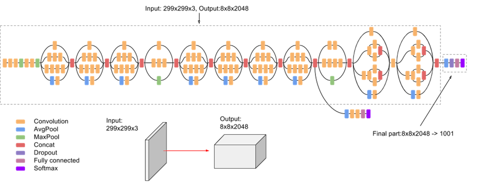
Image source: https://production-media.paperswithcode.com/methods/inceptionv3onc–oview_vjAbOfw.png
Results and Discussion:
Visualizations:
The model was able to classify the images into the 5 classes, namely :
- 0: No DR
- 1: Mild
- 2: Moderate
- 3: Severe
- 4: Proliferate DR
The visualization for Logistic Regression is :
The bar graph shows the classification of the retinal fundus images being classified into the stage of the diabetic retinopathy stages.
For Modified layers with VGGNet:
The improvement in accuracy with each epoch:
For Inception Model: Training and Validation Accuracy and Loss:


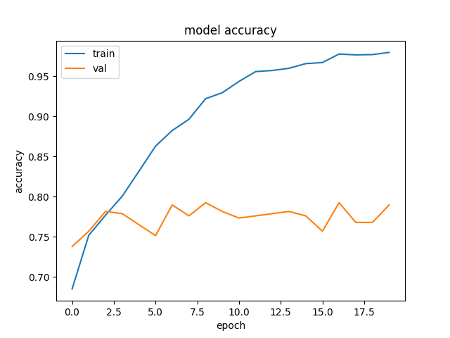
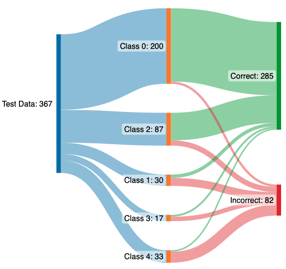
For ResNet Model:
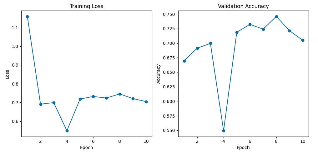
These visualizations display the validation accuracy and the training loss of the Resnet18 model. The visualization shows the impact that the change in epochs leads to improving the validation accuracy and the decrease in the training loss.
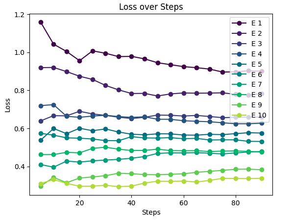
As the number of epochs and the number of steps increased the loss reduced and the plot above is superimposed with the 10 epochs that we used.
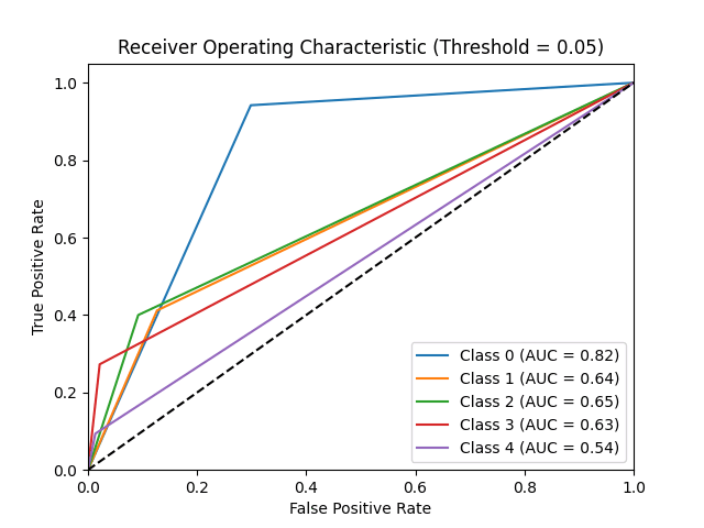
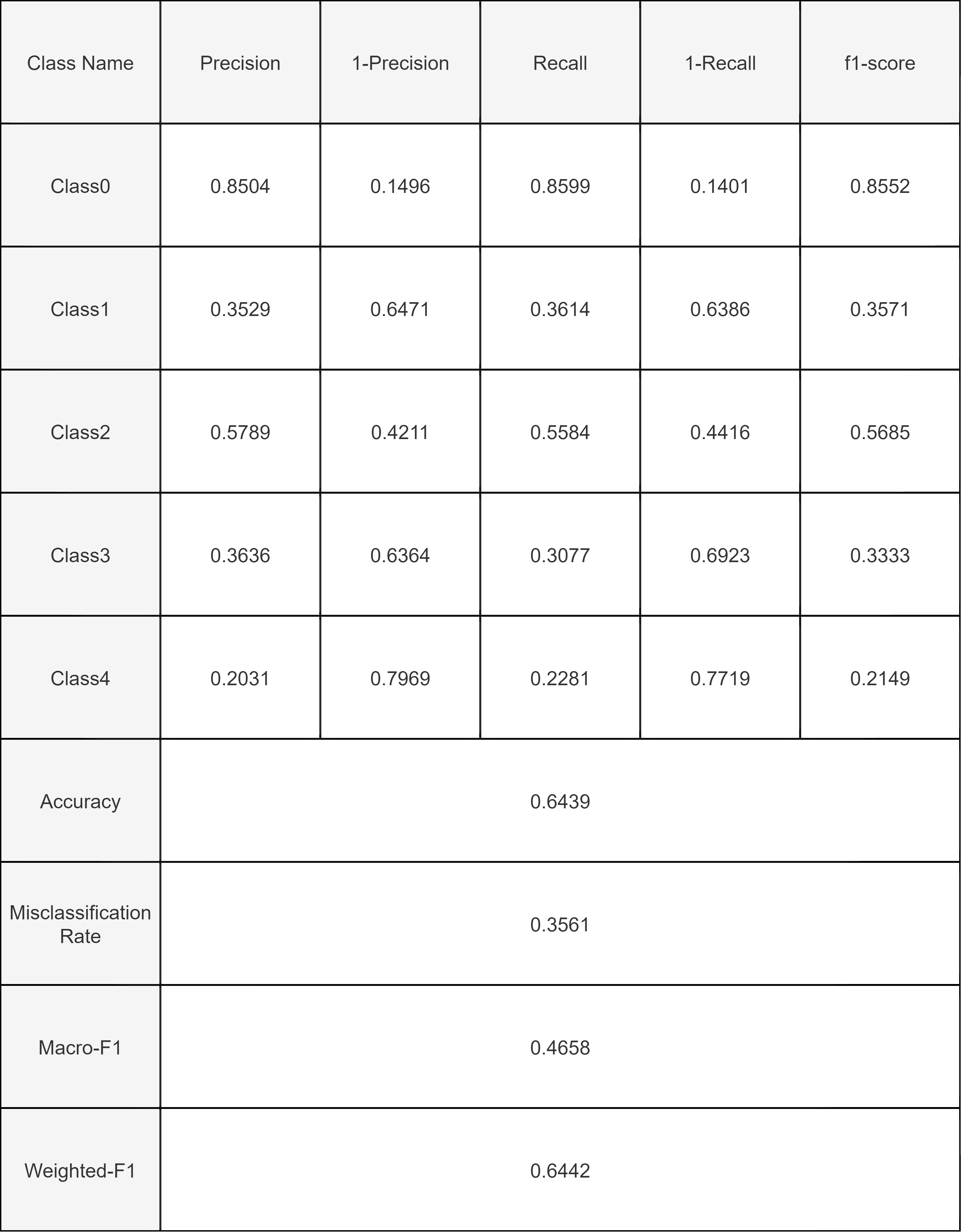
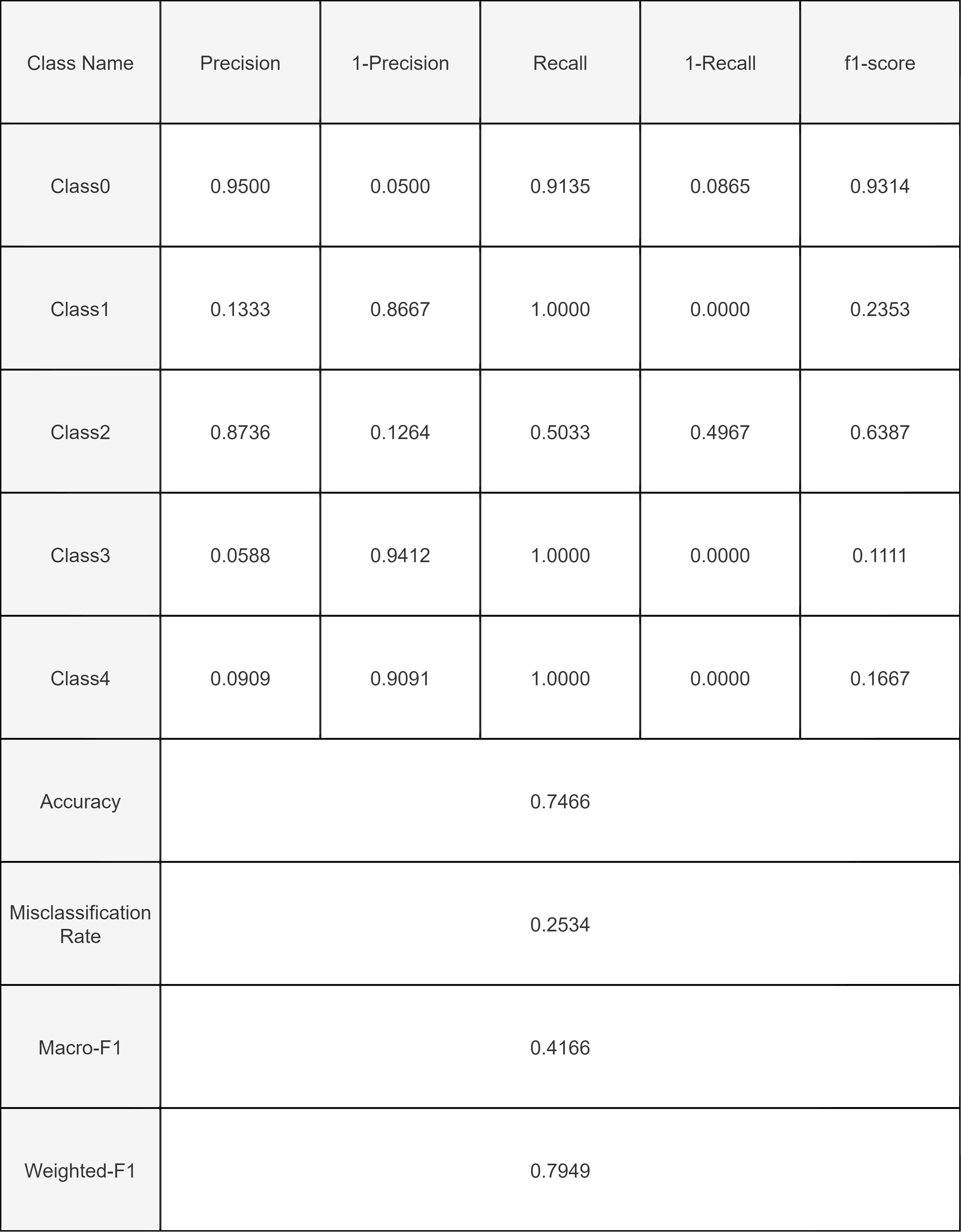
Quantitative Metrics:
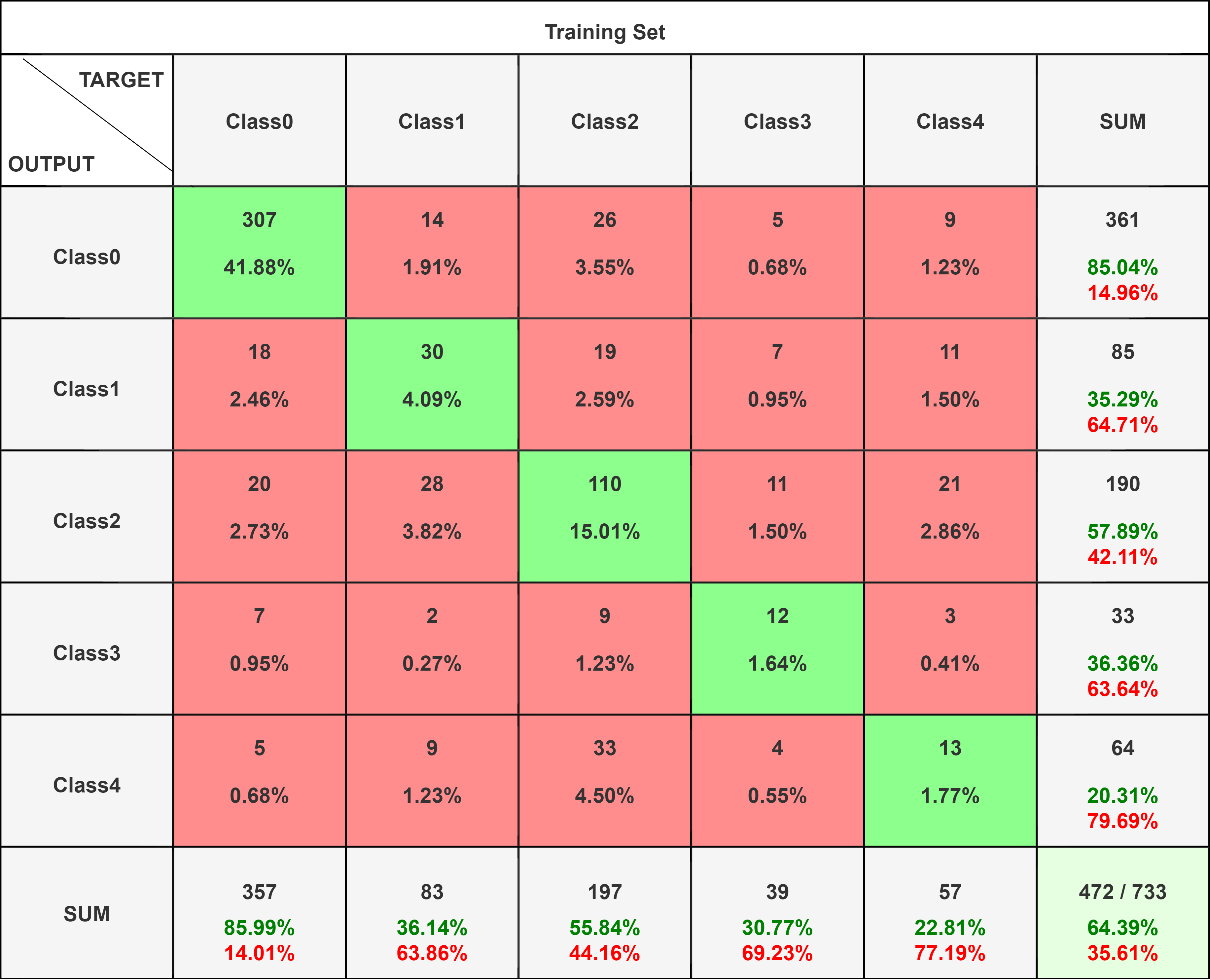
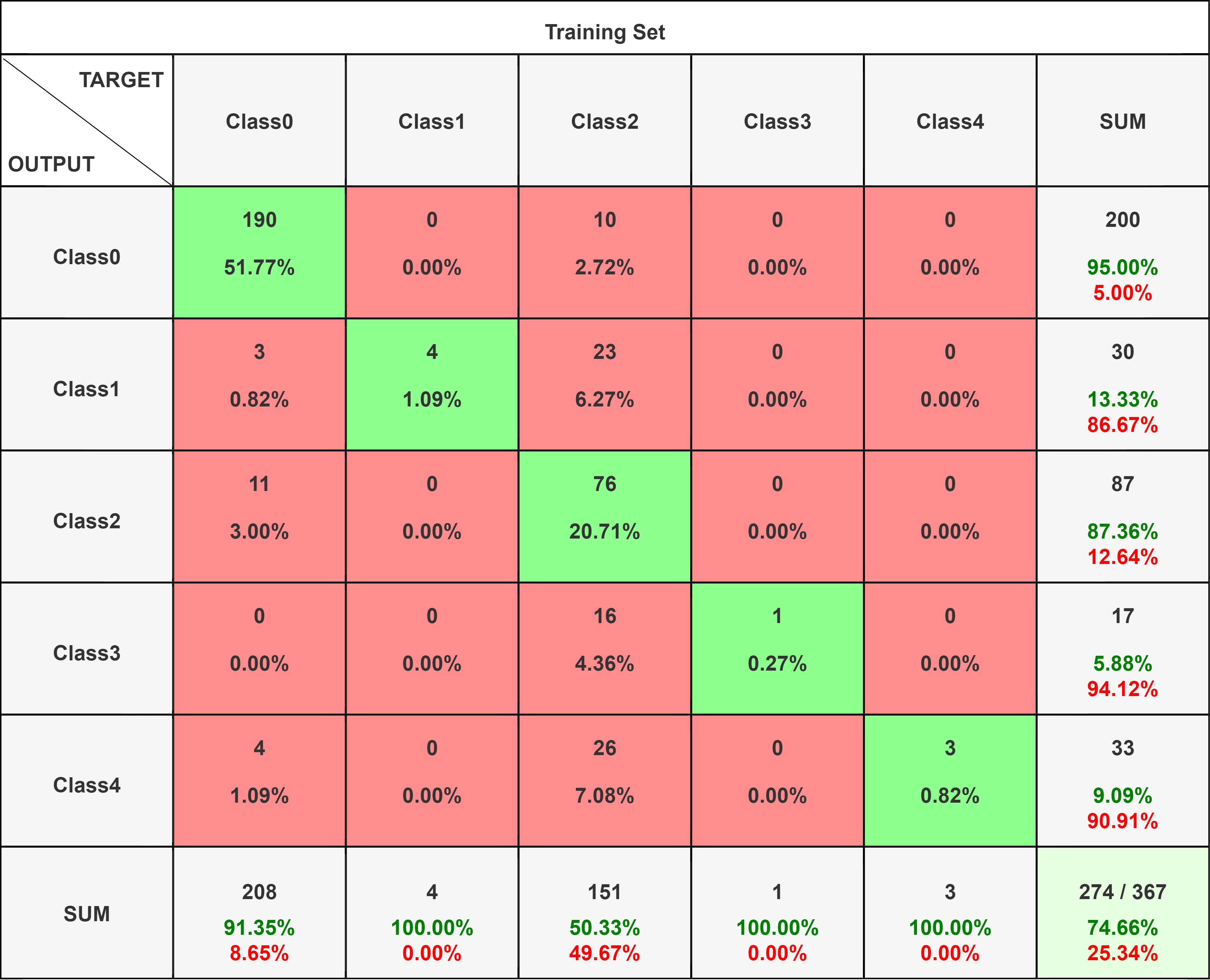
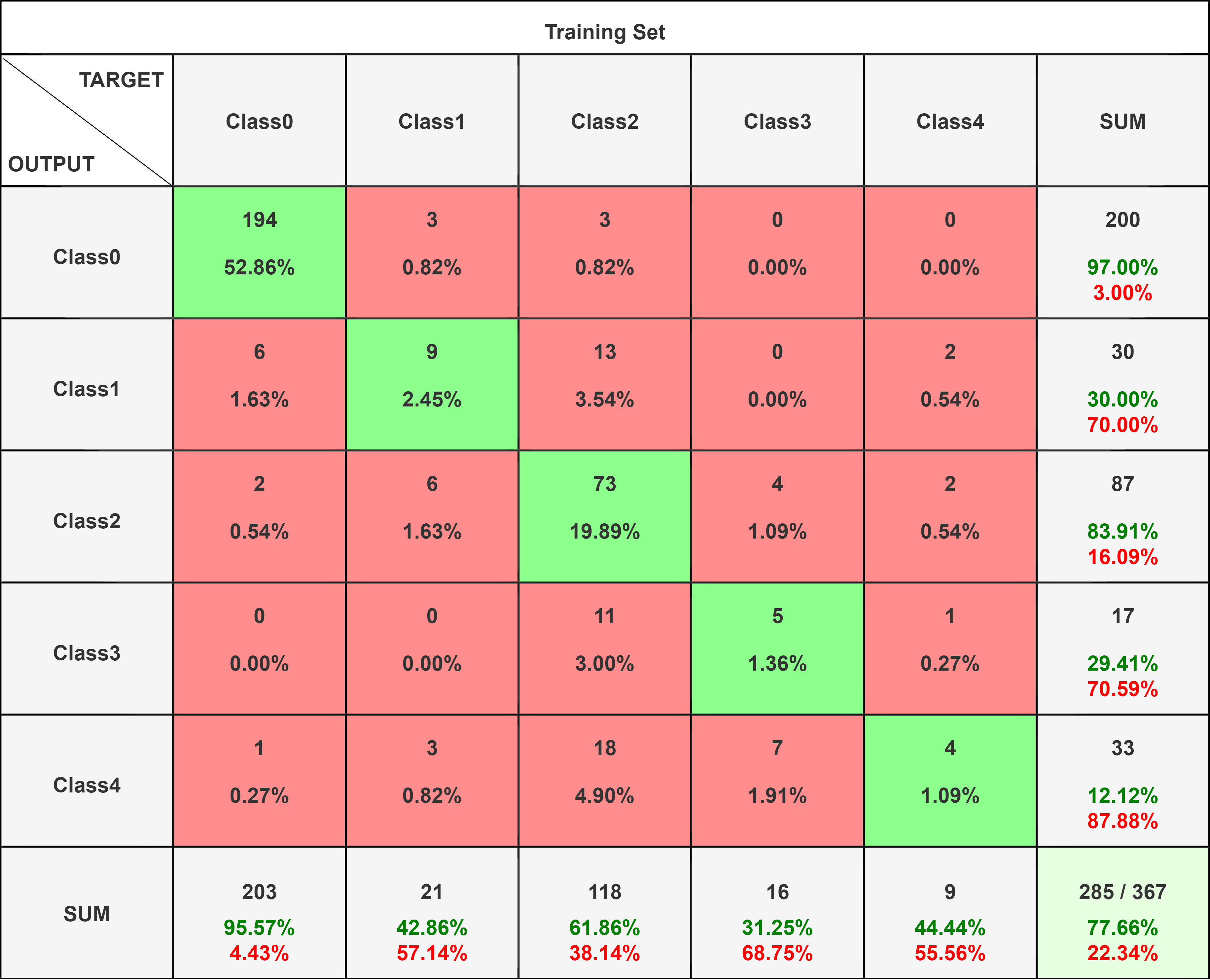
For our model, a good Qualitative Metrics is the Confusion Matrix. Confusion Matrix helps to give the comparison between the actual and the predicted values of the model.
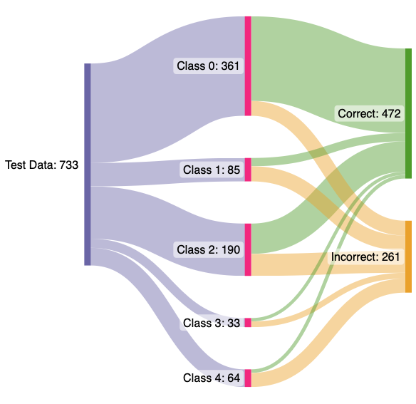
The confusion Matrix shows the True Positives, True Negatives, False Positives, False Negatives. The large number of True positive values for class 0 is due to excessive data of healthy class in the dataset.
The classes are defined as follows: ( DR is Diabetic Retinopathy)
- 0: No DR
- 1: Mild
- 2: Moderate
- 3: Severe
- 4: Proliferate DR
The five classes represent the stages of the Diabetic Retinopathy Disease.
For Logistic Regression:
For Inception Model:
For VGGnet Model:
For ResNet Model:
Precision measures of the accuracy of the positive predictions for the class made by the model. Mathematically it is : Precision = ((True Positives)/(True Positives+False Positives))
Recall, also known as sensitivity, it is the True Positive Rate. Mathematically it is: Recall = (True Positives)/(True Positives+False Negatives)
F1-score is Harmonic mean of precision and recall: Mathematically it is : (2 X Precision X Recall)/(Precision+Recall)
Analysis of Models:
The logistic regression on the data from PCA showed an accuracy of 64.39% on the test data. The model perfomed moderately well as the number of features (1092) is fairly high in comparision ot the number of datapoints (3662), which may have lead to including correlated features in the classification model.
The confusion matrix for the logistic regression shows that the F1 Score values are higher in classifying the retinal fundus images and this is in line to our accuracy. The model performs fairly well on the images and is able to classify the images on the severity of the disease based on the retinal fundus images. Additionally the low value of the False negatives and the False Positives in the confusion matrix show that the model performs well and the incorrect classifications are less.
We train the Resnet 18 model for 10 epochs with a batch size of 32, obtaining a test accuracy of 72.48%.
The VGGNet16 model with preloaded weights was trained for 20 epochs with a batch size of 64. A test accuracy of 77.6% was obtained on the unseen test data. The F1 scores are highest for classes 0 and 2. Classes 1 and 3 show similar values for their metrics (F1 score, precision and recall). This indicates that the model is good for classifying No DR and moderate DR, but shows poor performance for Proliferate DR.
The Inception-v3 model was trained for 50 epochs without pre-trained weights. A test accuracy of 74.66% was obtained on unseen data. Like the VGGNet16, the F1 scores are highest for classes 0 and 2. A thing to note is that the recall values of classes 1, 3 and 4 are 1, despite the precision being low.
Overall, across our models we see a good classification between DR and no DR, however, the performance when it comes to classifying the sub-classes of DR is not as great. It boils down to having less data for these sub-classes.
Comparison of Models:
Next Steps:
Having used different models and architectures to classify the data we had, we come to a conclusion that our models are able to perform well on the classes which have a good portion of datapoints. For example: Class 0 and Class 2 are classified more accurately than the other ones (evident from the sankey diagrams). To further improve the accuracy, more data should be collected and integrated to give the model enough variety to train on and extract as much varied information as possible. Further, more augmentations can be used in data pre-processing to feed the model with more variety.
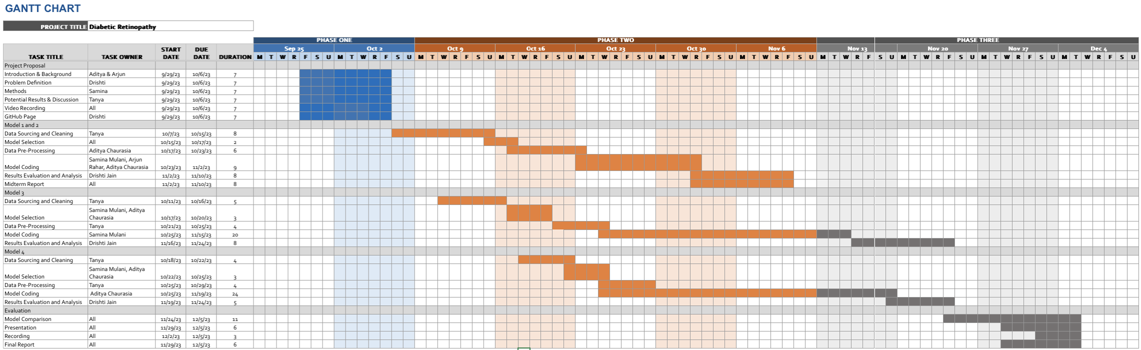
Gantt Chart
Contribution Table
| Task | Team Member |
|---|---|
| Introduction & Background | All |
| Problem Definition & Motivation | All |
| Model Comparison | All |
| Presentation | All |
| Recording | All |
| Final Report | All |
References:
- [1] https://www.ncbi.nlm.nih.gov/pmc/articles/PMC9924922/#ref1
- [2] Tymchenko, B., Marchenko, P., & Spodarets, D. (2020). Deep Learning Approach to Diabetic Retinopathy Detection. https://doi.org/10.48550/arXiv.2003.02261
- [3] Harry Pratt, Frans Coenen, D. M. B. S. P. H. Y. Z. (2016). Convolutional neural networks for diabetic retinopathy.
- [4] Rubina Sarki, Sandra Michalska, K. A. H. W. Y. Z. (2019). Convolutional neural networks for mild diabetic retinopathy detection: an experimental study. bioRxiv.
- [5] Carson Lam, Darvin Yi, M. G. and Lindsey, T. (2018). Automated detection of diabetic retinopathy using deep learning.
- [6] Yung-Hui Li, Nai-Ning Yeh, S.-J. C. and Chung, Y.-C. (2019). Computer-assisted diagnosis for diabetic retinopathy based on fundus images using deep convolutional neural network.
- [7] Abdulmajid Asiri, Sara AlBishi, Wedad AlMadani, Ashraf ElMetwally, Mowafa Househ (2019). The Use of Telemedicine in Surgical Care: a Systematic Review
- [8] Simon Mo, Ryan Cheng, Ian FangPay(2019). Attention to Convolution Filters: Towards Fast and Accurate Fine-Grained Transfer Learning